The Shropshire Hills Area of Outstanding Natural Beauty (AONB).
R
Published
November 15, 2023
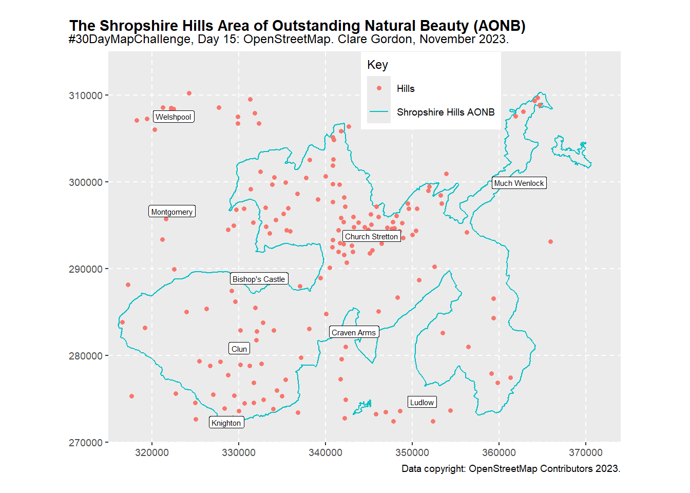
The Shropshire Hills Area of Outstanding Natural Beauty (AONB)
Playing with data and plotting in R again. Took ages, but I learnt a lot!
The Shropshire Hills AONB and the hills of South Shropshire.
Data
OpenStreetMap via osmdata package in R.
downloaded Shropshire Hills AONB boundary
Peaks within the bounding box
Places - towns only.
Tools
R with osmdata and ggplot2 packages.
What did I learn?
How to combine multiple layers in a plot
How to create a key for at least some of those layers - tried manual as well as auto.
How to label a points layer
What would I like to change?
Main thing is, I’d like to subset the hills to just within the AONB boundary, but the boundary is multiple line features, not a single polygon. So can I or would I need to, polygonise the lines in R?
Layout isn’t great…
Would look good with a hillshade or height layer behind it, but haven’t started looking at raster yet!!!
Process
Based on tutorial at https://jcoliver.github.io/learn-r/017-open-street-map.html
In the R notebook, but need to either include it, or summarise it here.
OpenStreetMap data in R
For Day 15 of the 30DayMapChallenge 2023.
Based on tutorial at: https://jcoliver.github.io/learn-r/017-open-street-map.html
Load required packages
library(osmdata)
Data (c) OpenStreetMap contributors, ODbL 1.0. https://www.openstreetmap.org/copyright
Subset peaks so only have those peaks within the AONB boundary
Not so easy, because the boundary is a line class, not a polygon feature…
Plotting downloaded layers
aonb_plot <-ggplot() +geom_sf(data = aonb_boundary$osm_lines,aes(colour ="Shropshire Hills AONB"))+geom_sf(data = peaks$osm_points,aes(colour ="Hills"))+geom_sf(data = places$osm_points,colour ="blue")+coord_sf(crs =st_crs(27700), xlim =c(315000, 374000), ylim =c(270000, 315000),datum =st_crs(27700), expand =FALSE)+geom_sf_label(data = places$osm_points, # Controls labels - in this case place names.aes(label = name), # field for the labelslabel.padding =unit(0.7, "mm"), # padding around the text - ie the white bitsize =2, # size of text - no idea what the units are!fill ="white")+labs(x =NULL, y =NULL, color ="Key",caption ="Data copyright: OpenStreetMap Contributors 2023.") +ggtitle("The Shropshire Hills Area of Outstanding Natural Beauty (AONB)", subtitle ="#30DayMapChallenge, Day 15: OpenStreetMap. Clare Gordon, November 2023.")+theme_grey(base_size =9) +# if don't set a theme, don't get coordinate grid...theme(plot.title.position ="plot",plot.title = ggtext::element_textbox_simple(face ="bold"),legend.position =c(0.63, 0.9),plot.margin =unit(c(0.5, 0.5, 0.5, 0.5), "cm"),panel.grid =element_line(color ="white", linewidth =0.4, linetype =2))# print the plotaonb_plot